Authors: @kanishk.chaturvedi @Nick_Van_Damme1
Introduction
In the fast-paced world of IoT, processing and analyzing data in real-time is crucial. With billions of devices generating vast amounts of data, leveraging Machine Learning (ML) is key to turning this information into actionable insights for smarter decisions and automation. However, the computational demands of ML models, especially when dealing with real-time data, necessitate robust and scalable solutions. This is where cloud-based hyperscalers like Amazon SageMaker, Microsoft Azure Machine Learning, and IBM Watson Studio come into play, offering powerful, flexible, and scalable platforms for hosting and executing ML models.
This article explores the integration of real-time IoT data from Cumulocity with these hyperscalers, highlighting the advantages and outlining a workflow for effective ML inferencing. By leveraging the combined strengths of IoT platforms and cloud-based ML services, businesses can unlock unprecedented value from their data, driving innovation and efficiency across industries.
Advantages of Hosting ML Models on Hyperscalers
Before moving on, let’s quickly understand the advantages of hosting ML Models on Hyperscalers!
Leading hyperscalers like Amazon SageMaker, Microsoft Azure Machine Learning, and IBM Watson Studio provide powerful platforms for hosting ML models, each offering distinct benefits for developers and organizations:
- Scalability: These platforms offer scalability, allowing for the adjustment of resources to meet the demand of ML workloads seamlessly. This ensures that models remain efficient and responsive, even in situations of very high data volumes.
- Managed Services: These platforms simplify the deployment and management of ML models by handling the underlying infrastructure. This enables developers to concentrate on refining models and deploying new features, rather than on maintenance tasks.
- No-Code Development: Platforms like AWS with Lookout for Equipment and IBM with AutoAI offer no-code development options, enabling users without deep technical expertise to create and deploy ML models. This democratizes ML, allowing a broader range of professionals to leverage AI for their specific needs, significantly accelerating innovation and implementation across various industries.
- Global Reach and Availability: With data centers spread across the globe, these platforms ensure that ML models are accessible with minimal latency, regardless of where the end-users or IoT devices are located. This global footprint is critical for applications requiring real-time insights from geographically dispersed data sources.
- MLOps Capabilities: These platforms also offer robust MLOps (Machine Learning Operations) capabilities, streamlining the entire process of model development, deployment, monitoring, and management. They provide tools for continuous integration and delivery (CI/CD) of ML models, automated testing, version control, and performance monitoring. This enables users to adopt best practices in DevOps for machine learning, ensuring that ML models are not only developed and deployed more efficiently but also remain reliable and accurate in production environments.
Workflow for ML Inferencing with Real-Time Cumulocity IoT Data
This section outlines a two-phase approach (as shown in Figure 1) to leveraging real-time IoT data for machine learning inferencing.

Phase 1: Model Training and Deployment
Data Preparation and Training: The foundation of this phase is the Cumulocity DataHub, which acts as a repository for aggregating and storing IoT data. DataHub plays a crucial role in off-loading data for extended intervals, making it particularly well-suited for training ML models. This data off-loading capability ensures that vast volumes of IoT data are efficiently managed and processed, allowing ML models to train on comprehensive datasets to recognize patterns and predict outcomes accurately. The training of these models is ideally performed on a hyperscaler platform, where advanced ML tools and substantial computational resources are readily available to accommodate the complexity and scale of IoT data.
Model Deployment: Once trained, the models are deployed over hyperscaler platforms. These platforms not only offer the essential scalability and advanced ML services for effective inferencing but also feature model managers for storing, managing, and continuously updating the ML models (more details on deployment capabilities of hyperscalers are here: Amazon Sagemaker, IBM Watson Studio, and Azure Machine Learning). In addition, these deployed models are accessible through simple REST endpoints, facilitating seamless integration and interaction with IoT applications and services.
Phase 2: Performing Real-Time Inferencing
The real-time inferencing process is illustrated in Figure 1, where data from IoT devices managed by Cumulocity is dynamically transmitted to the deployed ML model on the hyperscaler platform via secure API endpoints. This process involves Cumulocity’s Streaming Analytics capabilities, such as Analytics Builder or Event Processing Language (EPL), to define the logic for retrieving live data from devices. These analytics tools efficiently filter and forward relevant real-time or live data to the ML model’s endpoints for inferencing. The model then processes this data instantaneously, with the generated insights being promptly relayed back to Cumulocity for immediate action or in-depth analysis.
The major advantage of this two-phase approach is that on one hand, this approach allows us to leverage all the advantages of hyperscaler ML offerings for efficient inferencing on IoT data, while on the other, it eliminates the need for creating additional components like Microservices, thanks to the built-in capabilities of Cumulocity’s Streaming Analytics.
Example: Anomaly Detection in Wind Turbine Data
This section illustrates a practical application of the previously described workflow, focusing on a wind turbine scenario. In this example, a (simulated) wind turbine connected to Cumulocity IoT sends real-time data, including wind speed and power generated. We aim to use this data to train a machine learning model on Amazon SageMaker for anomaly detection, identifying potential issues in wind turbine operation.
Please note that the contents described here are only for demonstration purposes and are not intended for production scenarios.
Prerequisite
To follow this guide, you need the following:
- A Cumulocity (Trial) Tenant
- An AWS Cloud account
- IDE (e.g. Visual Studio Code)
- Familiarity with Python programming language
Step 1: Data Collection and Preparation
We start with a (simulated) wind turbine that has sensors to track how fast the wind is and how much power it is generating. This information is sent to Cumulocity IoT and forms the base of what we need to look at for our machine-learning model. To get our model ready, we gather data from the past three months, updating every minute. For simplicity, the data is offloaded into a simple CSV file in this demo. However, with the right access, this data could also be moved directly to DataHub to help get our model trained.
Step 2: Model Training on Amazon SageMaker
In the model training phase, we choose Amazon SageMaker for its powerful computational capabilities and leverage TensorFlow to design an Autoencoder model.
Autoencoders are particularly suited for anomaly detection because they excel at learning a normal operational baseline from data by compressing (encoding) the input into a lower-dimensional space and then reconstructing (decoding) it to match the original input as closely as possible. This characteristic makes them adept at highlighting deviations or anomalies from the norm when they attempt to reconstruct data that doesn’t fit the learned patterns.
Using the wind turbine data collected over three months, with updates every minute, we train our Autoencoder model on SageMaker. This training process enables the model to understand the typical patterns of wind speed and power generation, preparing it to identify instances that significantly deviate from these patterns, signaling potential anomalies.
# Import necessary Libraries
import pandas as pd
import numpy as np
import tensorflow as tf
from tensorflow.keras.models import Model
from tensorflow.keras.layers import Input, Dense
from sklearn.model_selection import train_test_split
from sklearn.preprocessing import MinMaxScaler
import matplotlib.pyplot as plt

# Load the dataset
# For simplicity, we use CSV File. With the right access, the data can also be loaded using DataHub
data_path = 'Data/measurements.csv'
data = pd.read_csv(data_path)

# Please make sure to clean the data (e.g. removing null or corrupted values) before transforming the data
# Scale the data to be between 0 and 1
scaler = MinMaxScaler()
data_scaled = scaler.fit_transform(data[['Wind.Speed.value', 'Power.Actual.value']])

# Split the data into training and test sets
X_train, X_test = train_test_split(data_scaled, test_size=0.2, random_state=42)

# Define the autoencoder model
input_layer = Input(shape=(2,))
# Encoder
encoded = Dense(128, activation='relu')(input_layer)
encoded = Dense(64, activation='relu')(encoded)
encoded = Dense(32, activation='relu')(encoded)
# Decoder
decoded = Dense(64, activation='relu')(encoded)
decoded = Dense(128, activation='relu')(decoded)
decoded = Dense(2, activation='sigmoid')(decoded)

autoencoder = Model(input_layer, decoded)
autoencoder.compile(optimizer='adam', loss='mse')

# Train the model
autoencoder.fit(X_train, X_train,
                epochs=50,
                batch_size=256,
                shuffle=True,
                validation_data=(X_test, X_test))
Following the training phase, we tested the model inferencing on new data. As shown in Figure 2, the left image presents the anomaly-free dataset used for training, while the right image displays the dataset, embedded with anomalies, used for inferencing. The accompanying graph effectively highlights how deviations from the established power curve, marked in blue, are accurately identified as anomalies, marked in red, by the model. It’s important to note that the right graph displays the values of wind speed and power normalized between 0 and 1, a necessary preprocessing step to match the autoencoder model’s expected input format.

Step 3: Model Deployment and Endpoint Creation
After training the Autoencoder model, we proceed to its deployment on Amazon SageMaker. SageMaker simplifies this process by offering the necessary libraries to efficiently load and deploy the trained model. Additionally, it facilitates the generation of a unique endpoint, ensuring seamless access to the model for real-time data analysis.
# Import necessary librraies
import boto3
import numpy as np
import os
import pandas as pd
import re
import sagemaker
from sagemaker.tensorflow import TensorFlowModel
from sagemaker.utils import S3DataConfig
import shutil
import tarfile

# Retrieve role, session and bucket details
role = sagemaker.get_execution_role()
sm_session = sagemaker.Session()
bucket_name = sm_session.default_bucket()

# Export the Autoencoder model developed in the previous step
autoencoder.save("export/Autoencoder/1")
with tarfile.open("autoencoder.tar.gz", "w:gz") as tar:
    tar.add("export")

# Upload the model to S3. Use your BUCKET_NAME
s3_response = sm_session.upload_data("autoencoder.tar.gz", bucket="<BUCKET_NAME>", key_prefix="model")

# Import model into SageMaker. Use your BUCKET_NAME
sagemaker_model = TensorFlowModel(
    model_data=f"s3://<BUCKET_NAME>/model/autoencoder.tar.gz",
    role=role,
    framework_version="2.12"
)

#Create endpoint. This step will generate a unique ENDPOINT for this model
predictor = sagemaker_model.deploy(initial_instance_count=1, instance_type="ml.m5.large")
For more information on setting up a unique Endpoint for a deployed model, please refer to the official guide of Amazon SageMaker.
Step 4: Integration with AWS Lambda for Pre- and Post-Processing
To ensure the live data is in the correct format for our deployed Autoencoder model on SageMaker, preprocessing steps are essential. AWS Lambda plays a crucial role here, allowing us to define logic that prepares the incoming data, ensuring the model can interpret it accurately. Once the model provides its prediction scores, Lambda aids in postprocessing, translating these scores into understandable labels that indicate normal operation or anomalies. Furthermore, AWS Lambda creates a unique endpoint for this entire process. This endpoint becomes the bridge for Streaming Analytics to send live data through, ensuring a seamless flow from data collection to actionable insights.
# Import necessary Libraries
import json
import boto3
import numpy as np

# Initialize a SageMaker runtime client
sagemaker_runtime = boto3.client('sagemaker-runtime')

# Hardcoded scaler parameters for WindSpeed and PowerActual
# This is usually calculated based on the training data
wind_speed_min = 1.0151
wind_speed_max = 25.8897
power_actual_min = 11.0
power_actual_max = 1799.0

# Define a threshold for anomaly detection
threshold = 0.1

def lambda_handler(event, context):
    # Parse the JSON-encoded 'body' key of the event object
    if 'body' in event:
        # Event body is JSON encoded, so parse it into a dictionary
        body = json.loads(event['body'])
    else:
        # Directly use event if testing from AWS console or if 'body' key is not present
        body = event

    # Safely access WindSpeed and PowerActual using the parsed body
    wind_speed = body.get('Wind.Speed.value')
    power_actual = body.get('Power.Actual.value')

    input_data = [wind_speed,power_actual]
    # Preprocess the input data
    # scaling based on predefined min/max values
    wind_speed_scaled = (wind_speed - wind_speed_min) / (wind_speed_max - wind_speed_min)
    power_actual_scaled = (power_actual - power_actual_min) / (power_actual_max - power_actual_min)

     # Prepare the scaled input data for the payload
    scaled_input_data = [[wind_speed_scaled, power_actual_scaled]]

    # Prepare the payload for SageMaker
    payload = json.dumps({"instances": scaled_input_data})

    # Invoke the SageMaker endpoint. Use the SageMaker <ENDPOINT> generated in the previous step.
    response = sagemaker_runtime.invoke_endpoint(
        EndpointName='<ENDPOINT>',
        ContentType='application/json',
        Body=payload
    )

    # Extract the result from the response and postprocess it
    result = json.loads(response['Body'].read().decode())
    predictions = result['predictions']

    # Here 'predictions' is a list of lists where each sublist contains model output
    predictions = np.array(predictions)

    # Calculate MSE using scaled input data and predictions
    mse = np.mean(np.square(scaled_input_data - predictions), axis=1)

    # Determine anomaly status based on the calculated MSE and predefined threshold
    anomaly_status = int(mse > threshold)


    #Print the anomaly_status
    return {
        'statusCode': 200,
        'body': json.dumps({'Anomaly': anomaly_status})
    }
For more information, please refer to the official guide of AWS Lambda.
Step 5: Real-Time Inferencing with Cumulocity Streaming Analytics
Following the setup of our AWS Lambda function, we leverage Cumulocity Streaming Analytics to handle real-time data processing efficiently. We write an EPL App, which captures live data from the (simulated) wind turbine sensors and routes it through the Lambda endpoint we established. The data undergoes preprocessing, prediction, and postprocessing seamlessly, allowing for the immediate identification of any anomalies. Furthermore, the processed insights trigger events (or alerts) within the Cumulocity platform, enabling prompt responses to potential issues detected by the machine learning model.
/**
* This application queries an external AWS Lambda URL (machine learning)
* to detect any anomaly in a simulated wind turbine data
*/

using com.apama.cumulocity.CumulocityRequestInterface;
using com.apama.correlator.Component;
using com.apama.cumulocity.Alarm;
using com.apama.cumulocity.Event;
using com.apama.cumulocity.Measurement;
using com.apama.cumulocity.FindManagedObjectResponse;
using com.apama.cumulocity.FindManagedObjectResponseAck;
using com.apama.cumulocity.FindManagedObject;
using com.softwareag.connectivity.httpclient.HttpOptions;
using com.softwareag.connectivity.httpclient.HttpTransport;
using com.softwareag.connectivity.httpclient.Request;
using com.softwareag.connectivity.httpclient.Response;
using com.apama.json.JSONPlugin;

/**
* Call external AWS Lambda URL
*/
monitor DetectAnomalies {

	CumulocityRequestInterface requestIface;

	action onload() {
		requestIface := CumulocityRequestInterface.connectToCumulocity();
		// Replace yourDeviceId with the value of your device id
		string yourDeviceId:= "891168235";
		listenAndActOnMeasurements(yourDeviceId, "sagemaker-1");
	}

	action listenAndActOnMeasurements(string deviceId, string modelName)
	{
		//Subscribe to the Measurement Channel of your device
		monitor.subscribe(Measurement.SUBSCRIBE_CHANNEL);

		on all Measurement(source = deviceId) as m {
			if (m.measurements.hasKey("c8y_Measurement")) {
				log "Received measurement" at INFO;
				dictionary < string, any > RECORD:= convertMeasurementToRecord(m);
				log "Sending record to AWS Lambda Function - " + JSONPlugin.toJSON(RECORD) at INFO;


				//Define the URL Parameters within the HTTPTransport
				//Mention here the URL of the Lambda endpoint
				HttpTransport transport := HttpTransport.getOrCreate("<LAMBDA_ENDPOINT>", 443);

				Request awsRequest:= transport.createPOSTRequest("/",RECORD);
				awsRequest.execute(awsHandler(deviceId).requestHandler);
			}
		}
	}

	action convertMeasurementToRecord(com.apama.cumulocity.Measurement m)
	returns dictionary < string, any >
	{
		dictionary < string, any > json := { };
		json["WindSpeed"] := m.measurements.
			getOrDefault("c8y_Measurement").
			getOrDefault("Wind.Speed.value").value;
		json["PowerActual"] := m.measurements.
			getOrDefault("c8y_Measurement").
			getOrDefault("Power.Actual.value").value;

		log "Sagemaker-1 - " at INFO;
		dictionary < string, any > inputs := json;
		return inputs;
	}


	event awsHandler
	{
		string deviceId;
		action requestHandler(Response awsResponse)
		{
			integer statusCode:= awsResponse.statusCode;
			if (statusCode = 200)
			{
				dictionary<string, any> outputs := {};


				any myresult := awsResponse.payload.data.getEntry("Anomaly");

				float anomaly := <float> myresult;

				string label;
				if(anomaly>0.0){
					label := "Anomaly";
				}
				else{
					label := "Normal";
				}

				//Create an Event with the correct Label
				send Event("",
						"[Sagemaker]ActivityRecognitionEvent",
						deviceId,
						currentTime,
						"[Sagemaker]Event Recognized as "+label,
						outputs) to Event.SEND_CHANNEL;
			}
			else
			{
				log "aws response :" +
					awsResponse.payload.data.toString()
					at INFO;
			}
		}
	}
}
Below is a screenshot of Cumulocity Device Management, listing the anomalies detected using the machine learning model by the above EPL app.

Conclusions and Next Steps
In conclusion, the integration of machine learning models with real-time IoT data, especially when leveraging the capabilities of hyperscalers offers transformative potential. The advantages of hosting ML models on hyperscalers—scalability, managed services, advanced ML tools, and global reach—provide a solid foundation for developing and deploying sophisticated ML solutions. Through the described workflow, we have showcased the seamless integration of real-time IoT data with ML endpoints outside of the Cumulocity platform for efficient inferencing, leveraging the built-in capabilities of Cumulocity without the need for creating any additional components, such as Microservices. Furthermore, by presenting a practical example, we’ve illustrated how this approach can be effectively applied to anomaly detection in wind turbine data, leveraging Amazon SageMaker for enhanced operational insights. The same approach can also be realized with other hyperscalers like IBM Watson Studio and Azure Machine Learning.
As a next step, our focus will be on embracing MLOps practices to ensure that machine learning models remain effective and efficient. By automating the end-to-end lifecycle of the ML models—from continuous training and deployment to monitoring and management—we can maintain high performance and adapt to new data seamlessly.
Addendum
This article shows that external inferencing with hyperscalers provides scalability and access to advanced ML tools, suitable for complex or resource-intensive models. However, some IoT use cases require low latency or ensuring data privacy which is not ideal for inferencing outside of Cumulocity.
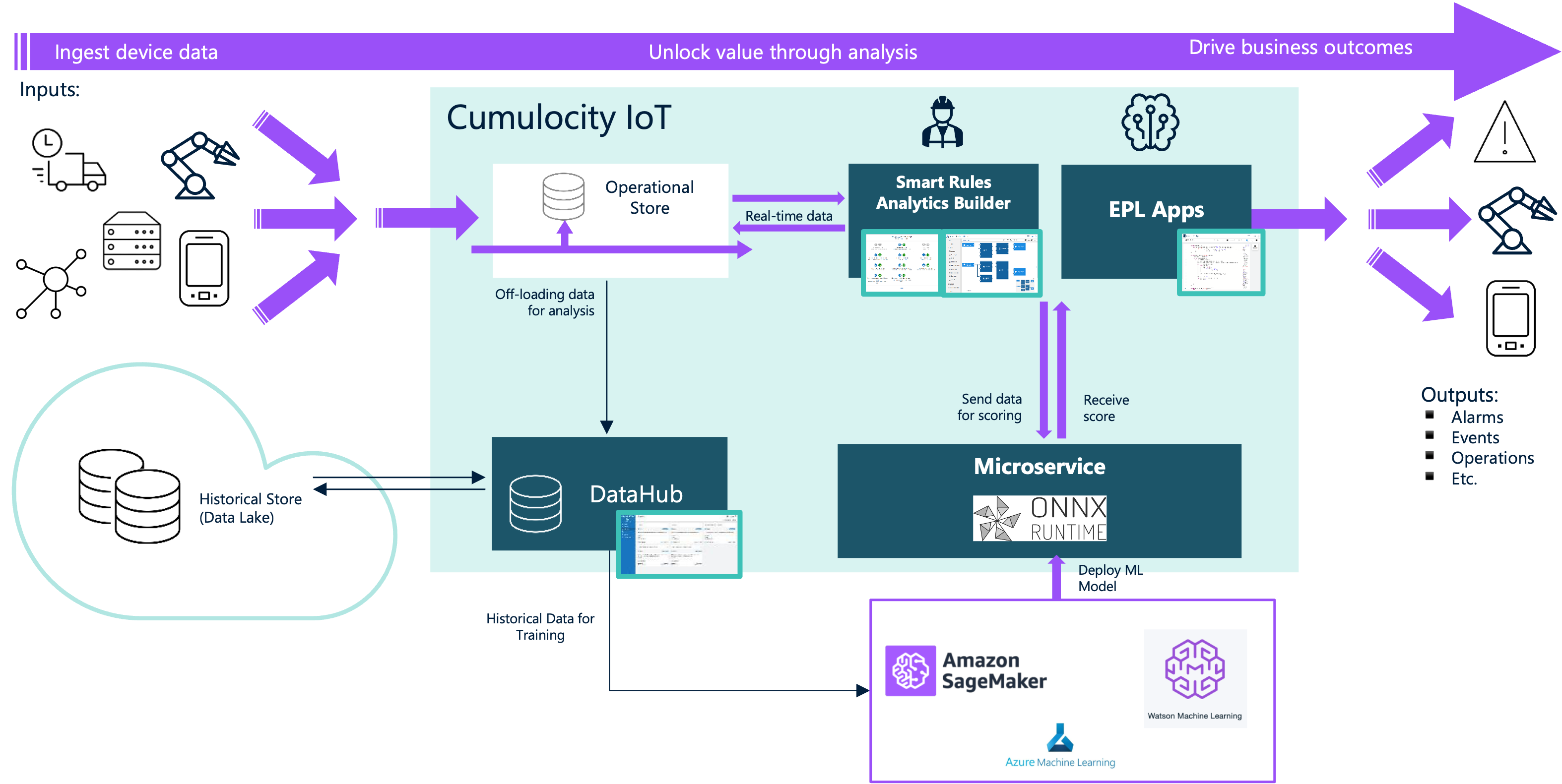
For scenarios where you’ve created an ML model within the Machine Learning tooling of the aforementioned hyperscaler and you do require close integration with IoT operations, you can opt to convert your model into an open format like ONNX. This format is compatible with Cumulocity’s in-built microservice architecture, enabling direct inferencing by leveraging an in-built ONNX RunTime microservice within the platform and feeding the real-time IoT data is directly to the internally deployed ML model, as shown in Figure 4. More details on this approach are described here.
Both inferencing approaches offer distinct advantages; the choice between external and internal inferencing depends on the specific requirements of the use case, including considerations of scalability, data sensitivity, and operational complexity.